Azure Quantum
Azure Quantum is a service offered by Microsoft through its cloud, Azure, or we can say it is the cloud quantum computing service of Azure, with a various set of quantum solutions and technologies. Azure Quantum provided to give an open, flexible, and future-proofed path to quantum computing.
It provides the best development environment to create quantum algorithms for multiple platforms at once .We can write the code once and run it with little to no changes against multiple targets of the same family which allows to focus our programming at the algorithm level.
This service has two distinct parts, Quantum Computing and Optimization. Both can be deployed by creating a Quantum Workspace resource in Azure.
Quantum computing
We can develop quantum algorithms using the Q# programming language and the QDK (Quantum Development Kit), with Quantum computing from Azure. Both Q# and QDK are open source. QDK includes specific libraries for chemistry, machine learning and qubit calculations. And we can use tools: Visual Studio, VS Code and Jupyter Notebooks.
The algorithms we implement can be executed on a small scale using the local QDK simulator, and we can also upload them to the cloud in the form of jobs, using a Quantum Workspace.
At the time of uploading a job we can choose which provider we want to run it in. Microsoft have providers that offer us simulators of quantum computers of greater capacity than our local and also real quantum computers with a few qubits.
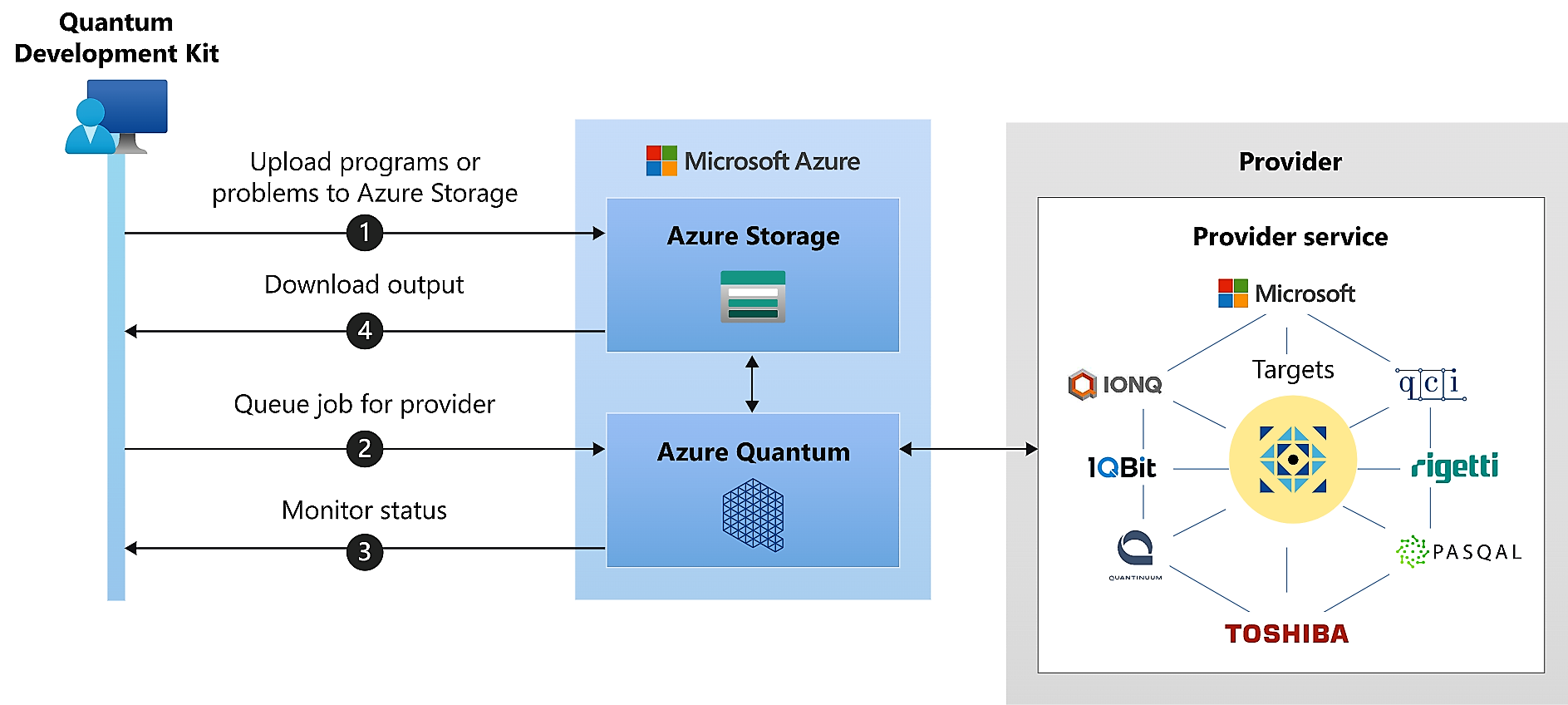
Quantum computing providers-
Choose the provider that best suits the characteristics of our problem and needs.
- Quantinuum: Trapped-ion system with high-fidelity, fully connected qubits, low error rates, qubit reuse, and the ability to perform mid-circuit measurements.
- IONQ: Dynamically reconfigurable trapped-ion quantum computer for up to 11 fully connected qubits, that lets you run a two-qubit gate between any pair.
- Rigetti : Gate-based superconducting processors.
- Pasqal: Neutral atom-based quantum processors operating at room temperature, with long coherence times and impressive qubit connectivity.
- Quantum Circuits,Inc: Full-stack superconducting circuits, with real-time feedback that enables error correction, encoding-agnostic entangling gates.
We don't have to compare the power of quantum computers by the number of qubits because it can be misleading. The Quantum Volume is somethinng we have to take in to the account .
So all thanks to Azure Quantum and Q# we can abstract from the hardware that will run our algorithm. However, it should be noted that the design of the algorithm can affect performance depending on the hardware used.
Optimization
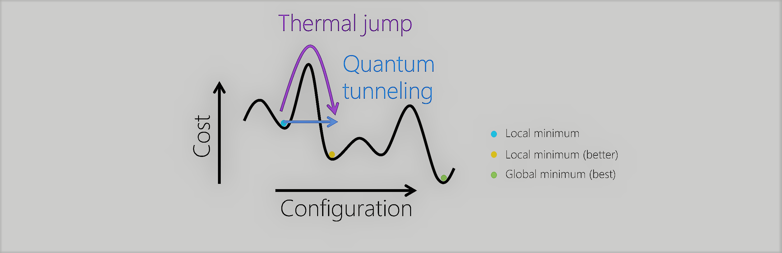
With Azure Quantum Optimization, we have access to optimization algorithms made by Microsoft and others. Optimization problems are solved by searching through the possible solutions. The best solution is the one with the lowest cost, although it is not always possible to find the best solution. A typical problem of optimization is the problem of the traveller (Travelling Salesman Problem), who tries to find the shortest route to travel through a set of cities and return to his home.
And also for solving combinatorial problems of simulated annealing but applying quantum mechanical effects.
Quantum annealing process could be created where the quantum device would use a very interesting property in quantum mechanics called quantum tunneling. This allows a quantum particle to jump barriers that, in our classical world, is not possible.
In order to use these algorithms, we must be able to define the problem to be solved in the terms of specification defined by the solvers. For this we will use the Python SDK: azure-quantum. These algorithms will run on classic hardware in Azure.
Currently,there are three optimization algorithm providers available, with the following solvers:
1- Microsoft QIO (Quantum-Inspired Optimization):
- Simulated annealing
- Simulated annealing (Parameter-free)
- Parallel tempering
- Parallel tempering (Parameter-free)
- Quantum Monte Carlo
2- 1QBit Optimization Platform:
- Tabu Search Solver
- Path-Relinking Solver
- PTICM Solver
3- Toshiba SQBM+
- Ising Solver
The advantage of using these algorithms inspired by quantum computing is that we can use them in real problems with improved speed, without having to wait for the advancement of quantum computers. And when the long-awaited quantum supremacy comes, we won’t have to change anything to take advantage of the new computing power.
Conclusion
Here, we have discussed how Microsoft, through Azure Quantum, provides us with the necessary tools to develop quantum algorithms both in simulators and in real quantum computers of a few qubits. In addition, it offers us some algorithms already implemented that we could use to solve optimization problems.
Let's try out some simulation.
Ex-1 Quantum entanglement with Q#
- Classical bits hold a single binary value such as a 0 or 1, the state of a qubit can be in a superposition of two quantum states, 0 and 1. Each possible quantum state has an associated probability amplitude.
- The act of measuring a qubit produces a binary result, either 0 or 1, with a certain probability, and changes the state of the qubit out of superposition.
- Multiple qubits can be entangled such that they cannot be described independently from each other. That is, whatever happens to one qubit in an entangled pair also happens to the other qubit.
We will see this in step wise manner-
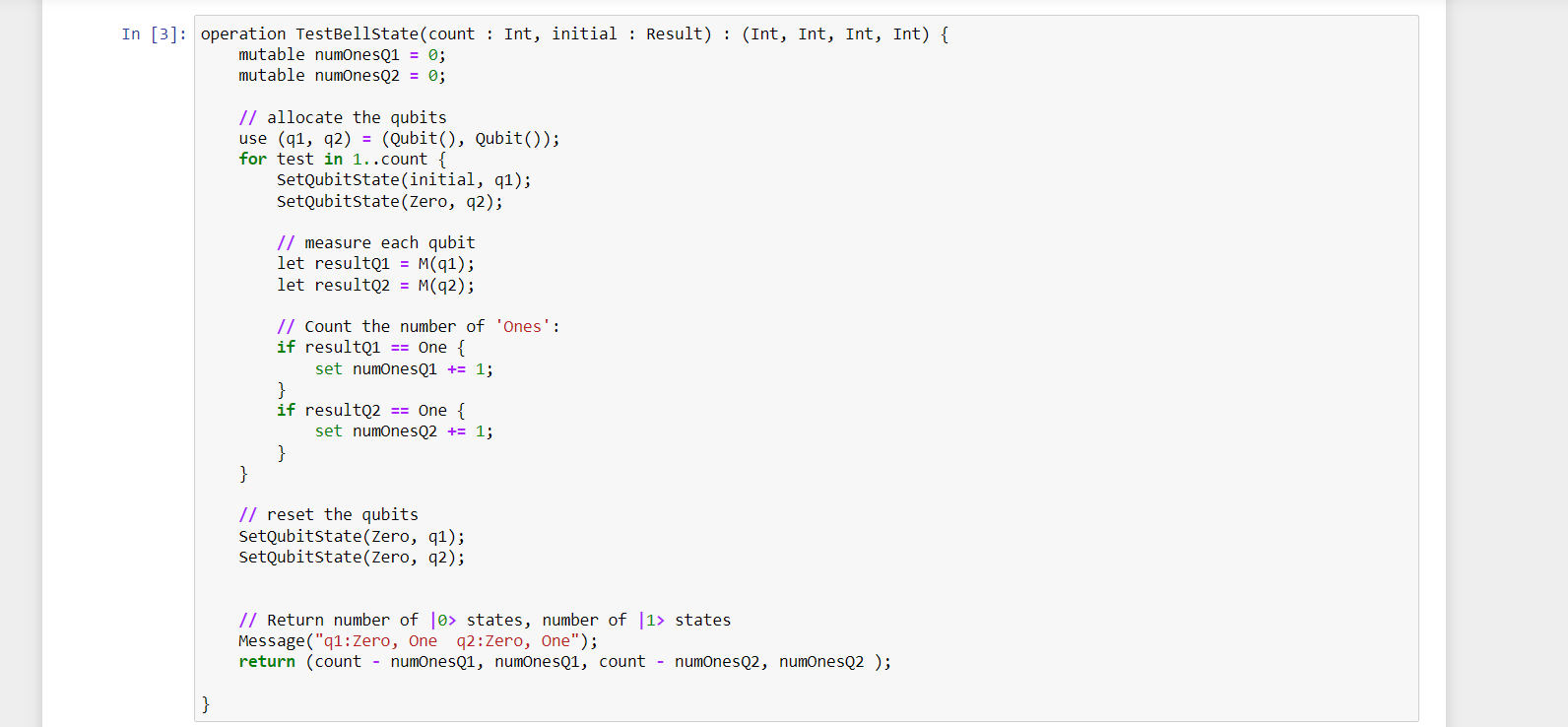
The TestBellState operation:
Test the measurement
- First we have to take two parameters: "count", which denotes the number of times to run a measurement, and "initial", which denotes the desired state to initialize the qubit.
- Then we will call the "use" statement to initialize two qubits.
- After that we will apply Loops for iteration "count".
And for each loop, it calls SetQubitState to set a specified "initial" value on the first qubit,again Calls "SetQubitState" to set the second qubit to a "Zero"state.
4- Then we will use "M" operation to measure each qubit.
5- And Stores the number of measurements for each qubit that return "One".
After the loop completes, it calls "SetQubitState" again to reset the qubits to a known state (Zero) to allow others to allocate the qubits in a known state. This is required by the "use"statement.
6- Finally, it uses the "Message" function to display a message to the console before returning the results.
Input:
msg : String
The message to be reported.
Output : Unit*
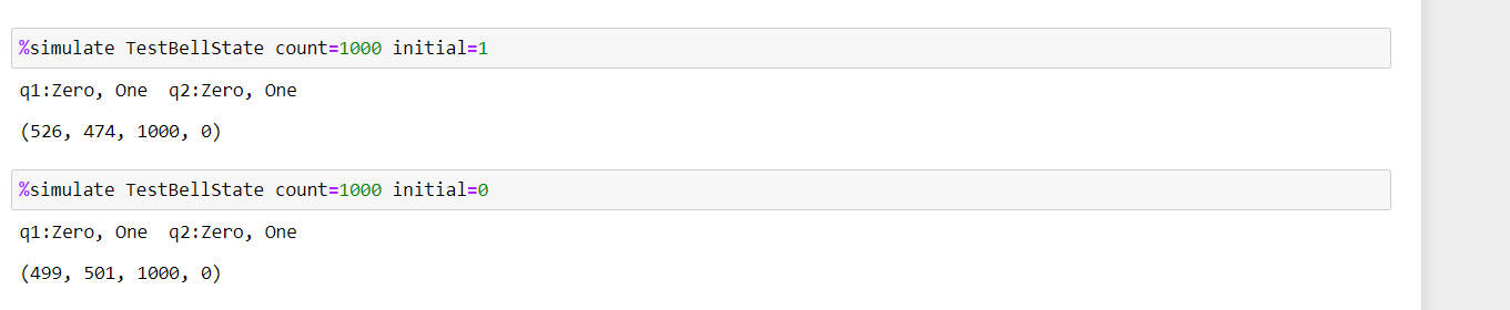
7- Test the code
Test the code up to this point to see the initialization and measurement of the qubits.
To run the "TestBellState" operation, you use the "%simulate" magic command to call the Azure Quantum full-state simulator. Here we need to specify the "count"and "initial" arguments,
Since the qubits has not been manipulated yet, they have retained their initial values:

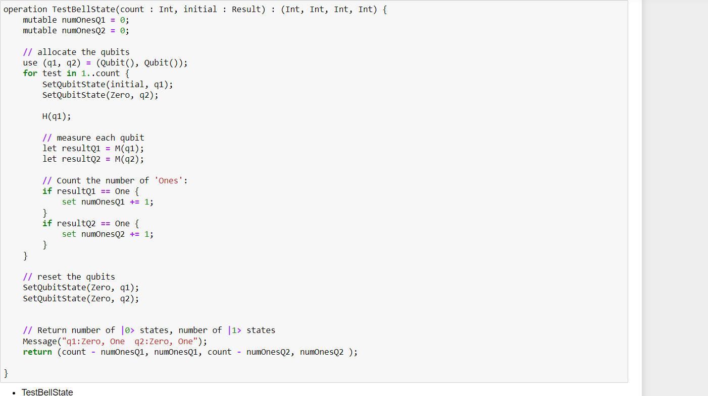
Put a qubit in superposition
Before entangling the qubits, you will put the first qubit into a superposition state, where a measurement of the qubit will return Zero 50% of the time and One 50% of the time. Conceptually, the qubit can be thought of as being in a linear combination of all states between the Zero and One.
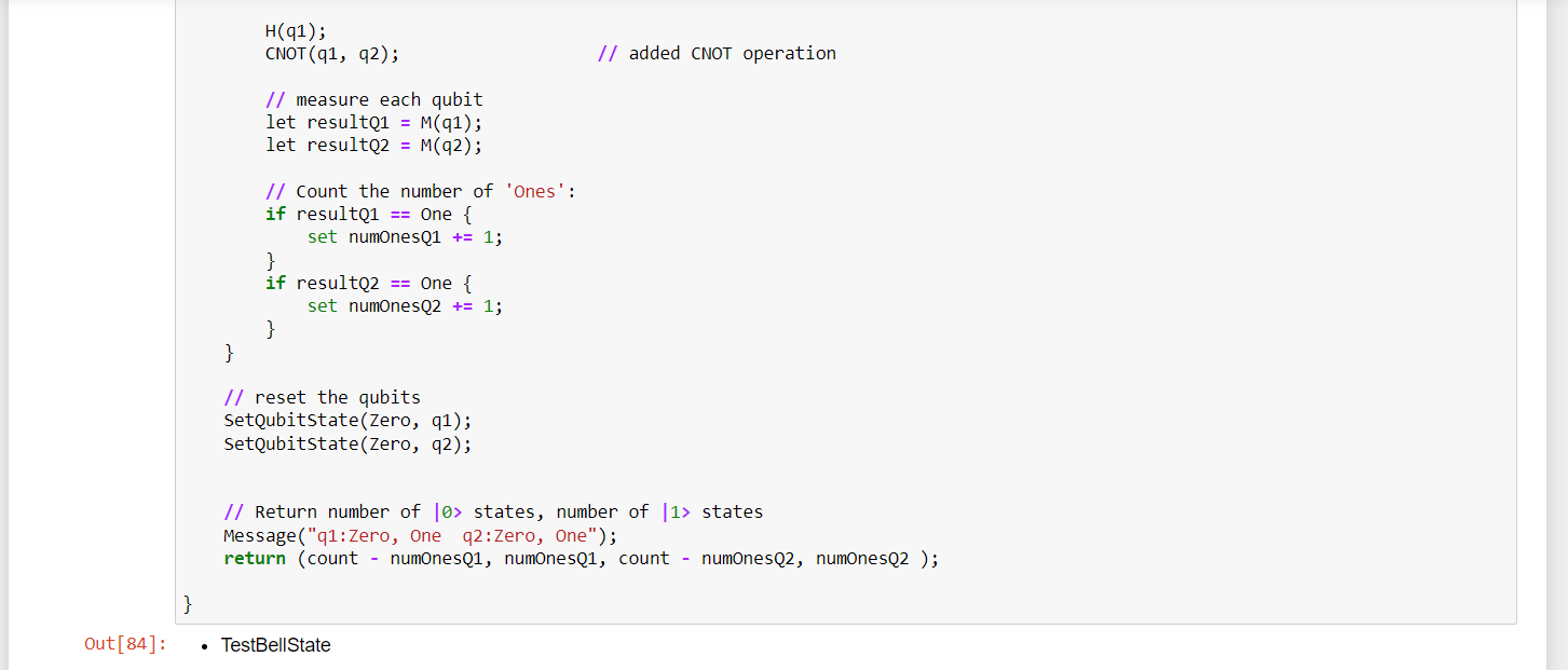
To put a qubit in superposition, Q# provides the H or Hadamard, operation.
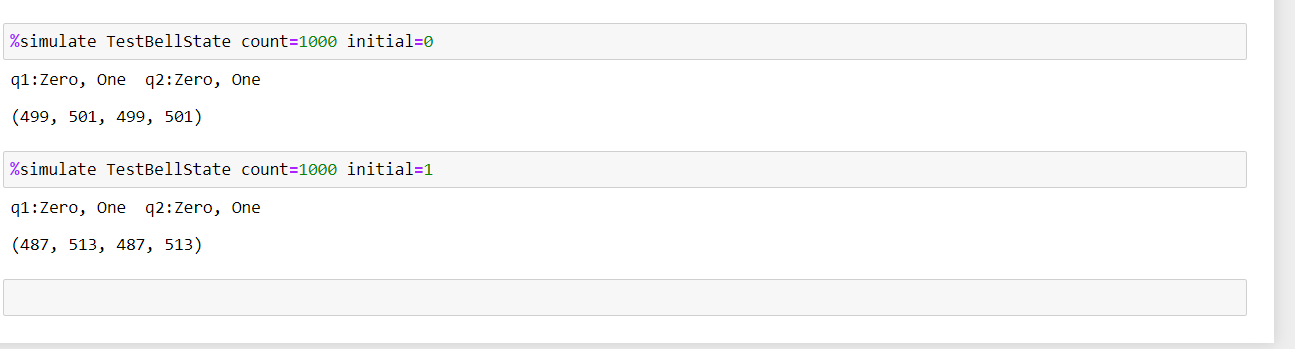
Entangle two qubits
Entangled qubits are connected such that they cannot be described independently from each other. That is, whatever operation happens to one qubit in an entangled pair, also happens to the other qubit.
To enable entanglement, Q# provides the CNOT operation, which stands for Controlled-NOT.
Ex-2 Write and simulate qubit-level programs in Q#
Let's simulate a basic quantum program that operates on individual qubits.
Quantum Fourier Transform(QFT)
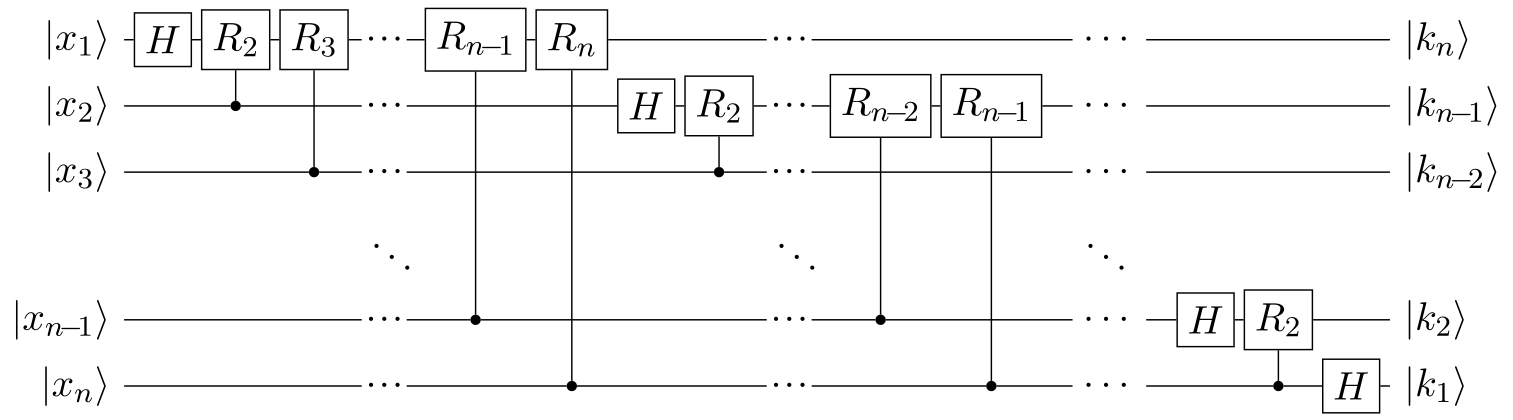
The quantum Fourier transform is a part of many quantum algorithms.The quantum Fourier transform can be performed efficiently on a quantum computer with a decomposition into the product of simpler unitary matrices.
The discrete Fourier transform on 2^n amplitudes can be implemented as a quantum circuit consisting of only Hadamard Gates and controlledphase shift gates, where n is the number of qubits.
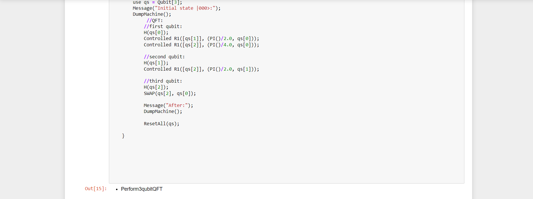
Step 1: define the Perform3qubitQFT operation
Step 2: allocate a register of three or four qubits with the use keyword
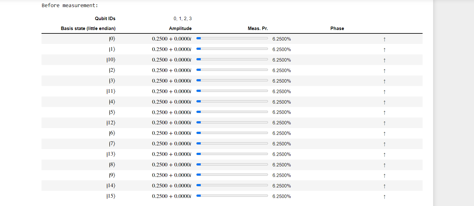
Step3: we can verify their allocated state by using DumpMachine ,which prints the system's current state to the console.
Step4: a) Applying single-qubit
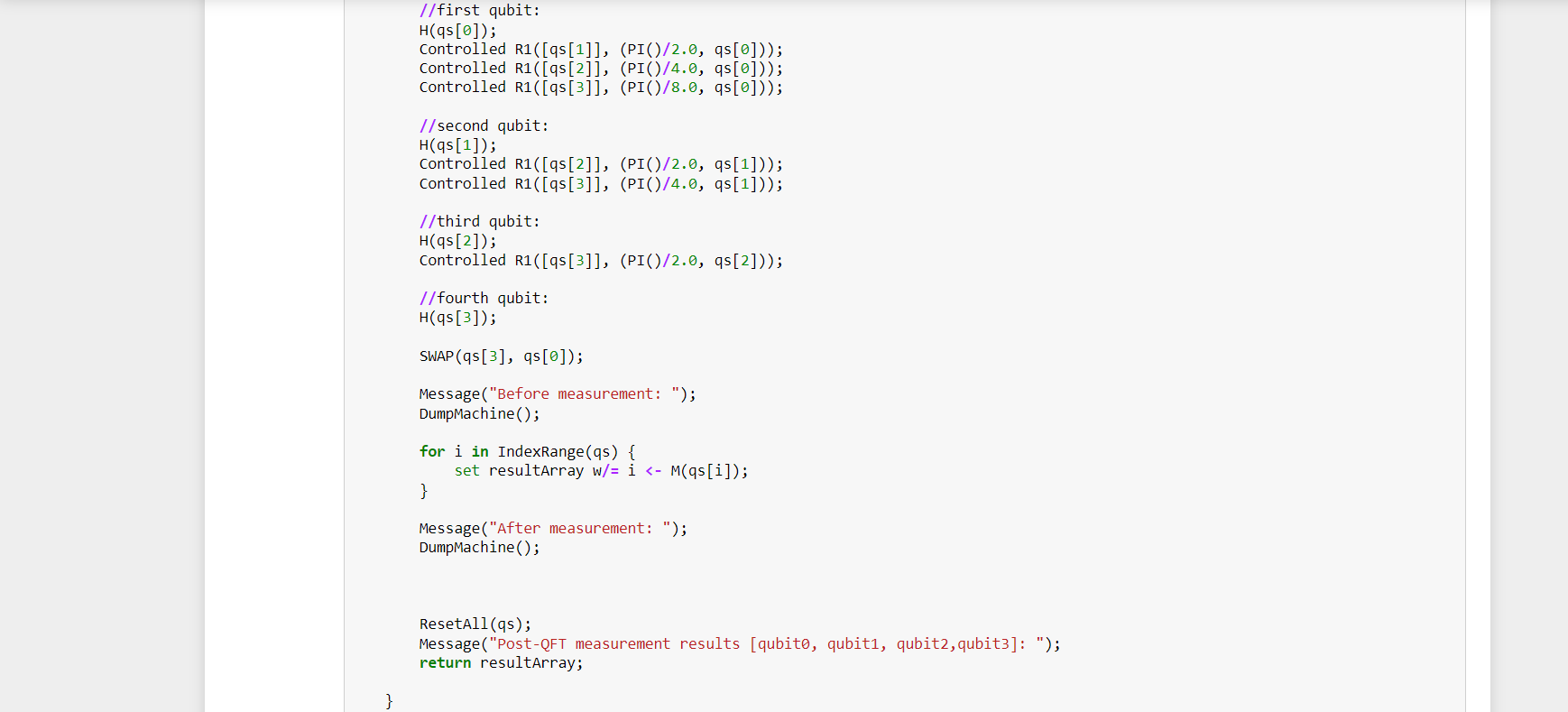
The first operation applied is the H (Hadamard) operation to the first qubit
To apply an operation to a specific qubit from a register , use standard index notation. So, applying the H operation to the first qubit of the register qs takes the form
b) Controlled operations
The QFT circuit consists primarily of controlled R1 rotations. An R1(Theta,qubit) .
So the R1 operations will act on the first qubit (and controlled by the second and third qubits),and so on.
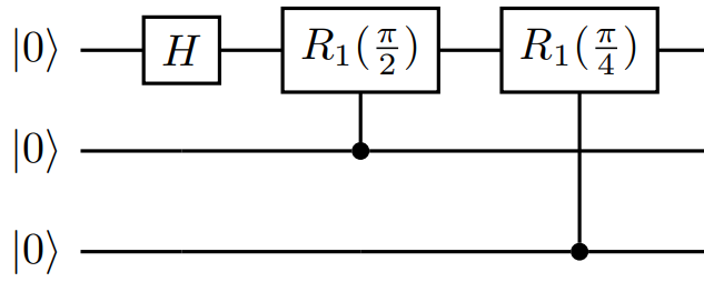
The PI() function is used to define the rotations in terms of pi radians.
After applying the relevant H operations and controlled rotations to the second and third qubits / second,third and fourth qubits.
Step 5 : Then apply a SWAP operation to complete the circuit.
This is necessary because the nature of the quantum Fourier transform outputs the qubits in reverse order.
Step 6: Deallocate qubits
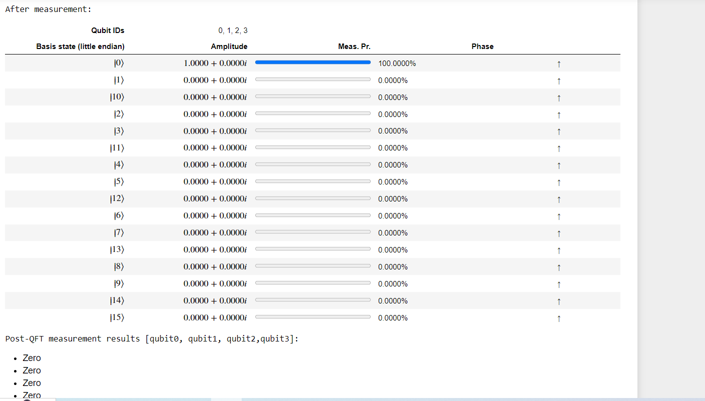
The last step is to call DumpMachine() again to see the post-operation state, and to deallocate the qubits. The qubits were in state |0⟩ when we allocated them and need to be reset to their initial state using the ResetAll operation.
Step 7: Test the operation
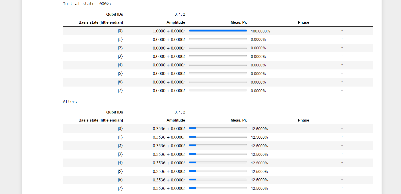
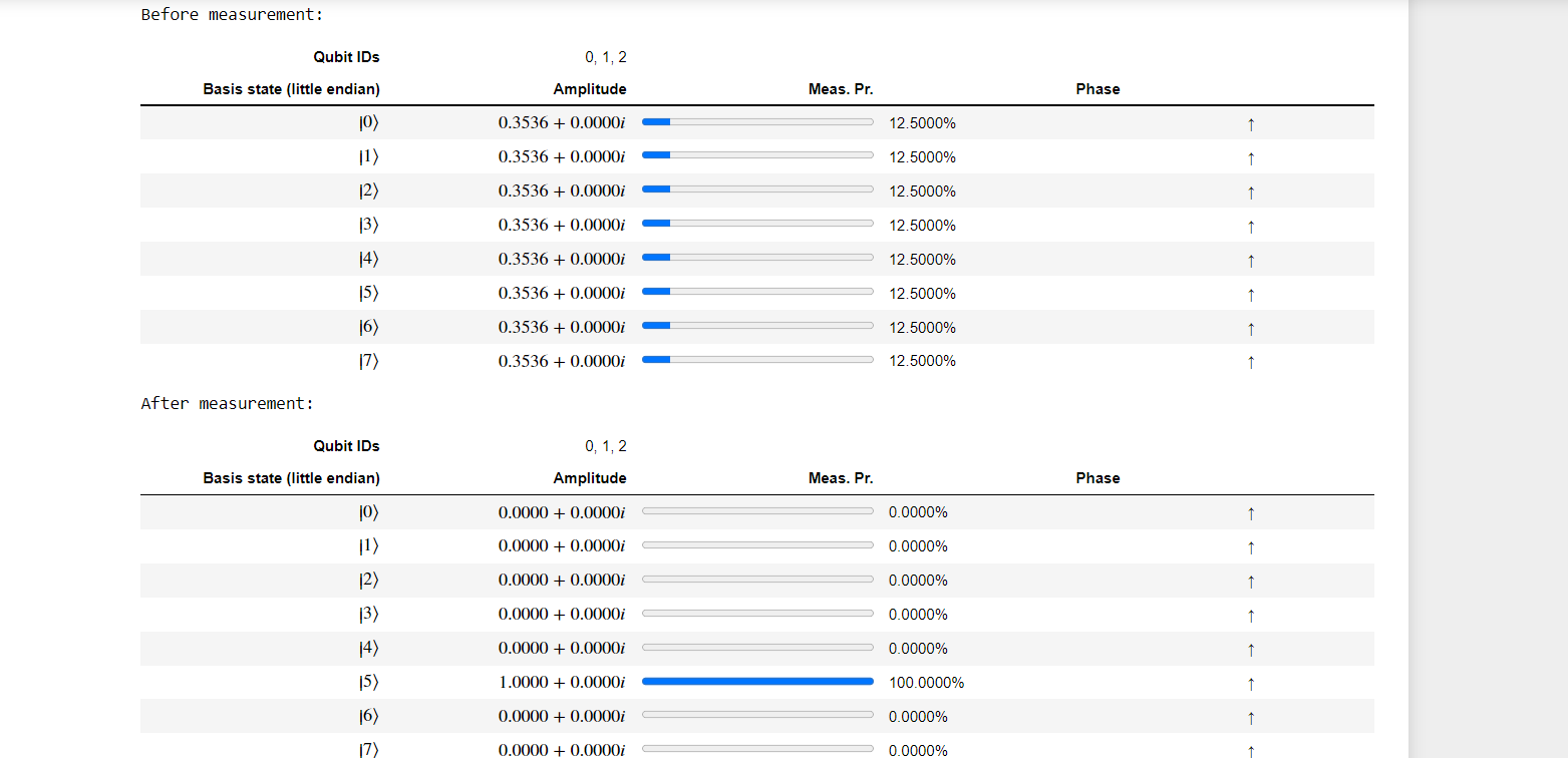
Step 8: Understanding the output
When called on the full-state simulator, DumpMachine() provides these multiple representations of the quantum state's wavefunction.
The first row provides a comment with the IDs of the corresponding qubits in their significant order.
The rest of the rows describe the probability amplitude of measuring the basis state vector |i⟩ in both Cartesian and polar formats.
a) With 3 Qubits
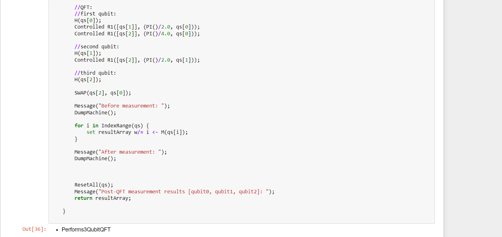
Now let's Modify the operation
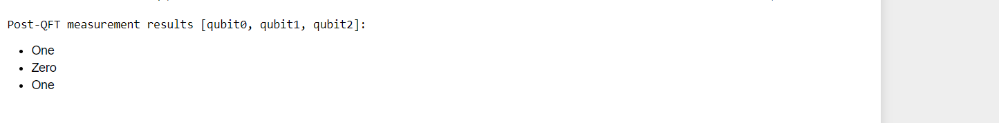
Firstly Define and initialize Result[] array
Lastly , Perform measurements in a for loop and add results to array
With all three qubits measured and the results added to resultArray, you are safe to reset and deallocate the qubits as before.
b) With 4 qubits