Quantum Machine Learning(QML) Technique-

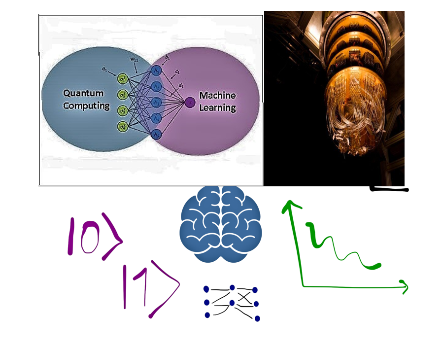
Why Quantum Machine Learning?

Machine learning is being applied to different sectors, from military to aerospace, from finance to healthcare and from agriculture to manufacturing.Since these algorithms consist of billions of parameters so it become hard to train. Quantum computers promise to solve such problems with the use of current computing technologies. And also, its ability to compute multiple states simultaneously enables it to perform an infinite number of superposed tasks parallelly. So this power of Quantum Computing promises to improve and advance the machine learning techniques.Classical computers based on sequential information processing but quantum computing uses the properties of quantum physics: superposition, entanglement, and interference.

Quantum computing requisites a whole new set of algorithms. Algorithms that encode and use quantum information. This introduces Machine learning Algorithms.

How Does Machine Learning Work?

There are countless numbers of machine learning algorithms out there. But each and every of these algorithms has three major factors:

• The representation part : It consists of rules, instances, decision trees, support vector machines(SVM), neural networks, and others.

• The evaluation  part: Its function to evaluate algorithm parameterizations.For example accuracy, prediction and probability, cost, margin, entropy, and others.

• The optimization part: It is the way of generating algorithm parameterizations. It is  basically called as the search process – for instance, combinatorial optimization, convex optimization, and constrained optimization.

QUBO

Quadratic unconstrained binary optimization (QUBO),also known as unconstrained binary quadratic programming.It combines various combinatorial optimization problems with a vide range of applications in finance and economics to machine learning that uses the applied optimization models in the quantum computing domain.

Ising Model

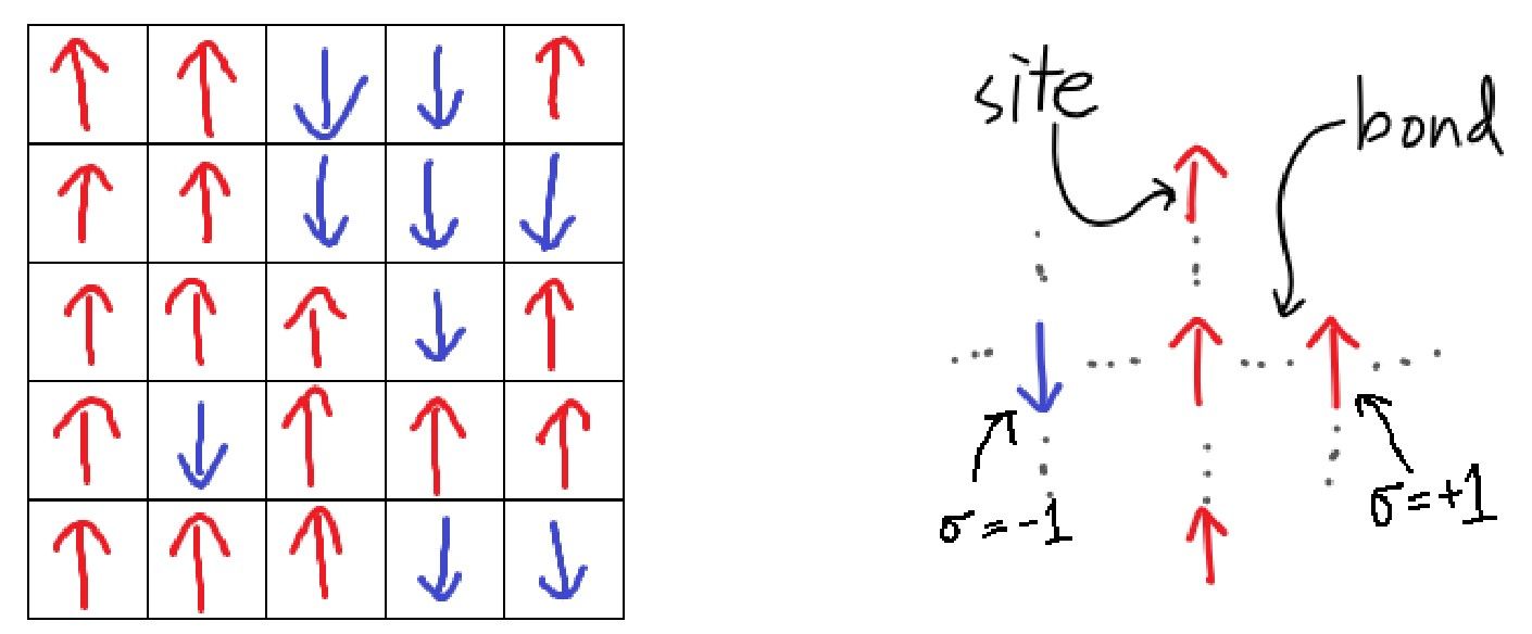
The importance  of QUBO model lies in its capacity to bound several  model in combinatorial optimization.The Ising model is a theoretical mathematical model of ferromagnetism about statistical mechanics, which plays an important role in physics. The model uses discrete variables representing the magnetic dipole moments of spin states (which are either +1 /–1).And the spin states are organized as a lattice so that each spin can interact with its neighbors.

The Ising model does not correspond to an actual physical system.It is  a huge(square) lattice of sites, where each site can be in one of two states.Each site is labeled with an index i,and the two states are referred to as –1 and +1.

For example,when we state that spin σi = − 1, we mean that the i-th site is in the state –1. Magnetic behavior can be understood by thinking of each atom as a spin, pointing up or down.

The energy of the Ising model is defined in terms of its Hamiltonian.

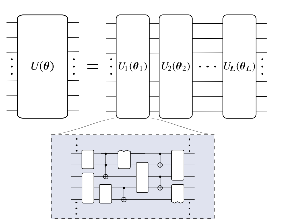
Variational Quantum Circuits(VQC)

The Schrödinger equation can be used to study and simulate the behavior and the evolution of a single quantum particle.But the real-world phenomena are dependent on the interactions between many different quantum systems.Hence,the study of many-body Hamiltonians that model physical systems are the major concern of condensed matter physics, molecular dynamics, and modeling. Variational methods are of major importance in quantum machine learning practice.Many-body Hamiltonians are essentially hard to model and investigate on classical computers due to the Hilbert space's features, whose dimension grows exponentially with the number of particles in the system.

It may seem attractive to use quantum computers for problems related to many-body physics and molecular simulations, reality is near-term quantum computers are far from being perfect and suffer from imperfections.

So the preparation of quantum states using low-depth quantum circuits is one of the most promising near-term applications of small quantum computers, especially if the circuit is short enough and the fidelity of gates are high enough to be executed withot quantum error correction.And such quantum state preparation can be used in variational approaches, optimizing parameters in the circuit to minimize the energy of the constructed quantum state for a given problem Hamiltonian.

The primary idea is to run a short sequence of gates where some gates are parametrized.The process then reads out the result, and adjusts the parameters on a classical computer,in turn repeats the calculation with the new parameters on the quantum hardware.In this way, an iterative loop is created between the quantum and the classical processing units, creating classical-quantum hybrid algorithms .

These algorithms are called variational to reflect the variational approaches to changing the parameters.

So such quantum state preparation is use to minimize the energy of the constructed quantum state for a given problem Hamiltonian that can be used in variational approaches, optimizing parameters in the circuit.For these reasons, variational circuits are also known as parameterized quantum circuits .

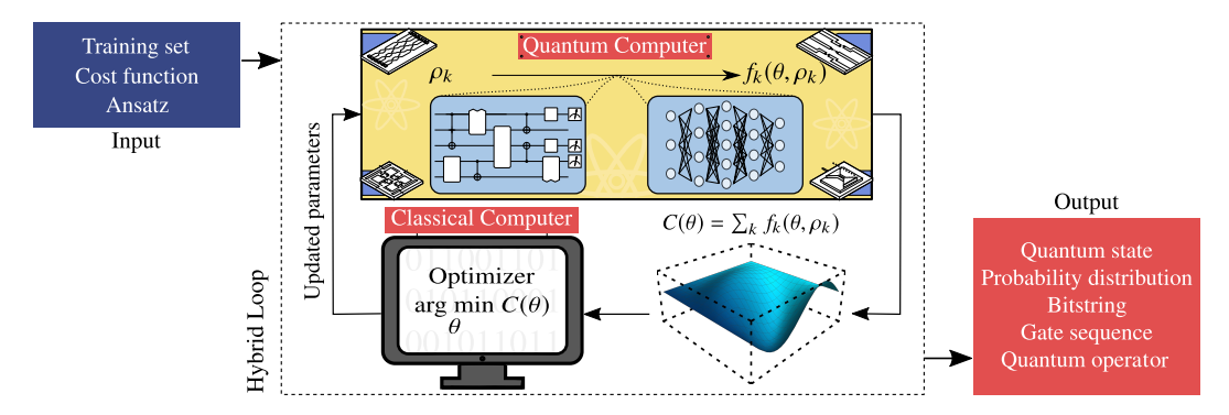
The following are VQA inputs: a cost function C(θ) encoding the solution to the problem, an ansatz whose parameters are trained to minimize the cost, and optionally (if required), a set of  training data used during the optimization. At each iteration of the loop, a quantum computer efficiently estimate the cost. The output of this information is fed into a classical computer that makes  the use of the power of optimizers to handle the cost derivatives and solve the optimization problem in equation.Once a termination condition is met, the VQA estimates an output of the solution to the problem. The form of the output depends on the precise task.

The cost functions and the choice of  ansatz both are important for VQAs.The form of the ansatz define the parameter and they can be trained to minimize the cost.The specific structure of Ansatz generally depends on the task Some other ansatz architectures are generic and independent of the problem, meaning they can be used even when no relevant information is readily available.

Variational Quantum Eigensolver (VQE)/ The Variational Quantum Eigensolver (VQE) is a hybrid quantum-classical algorithm, a tool which is use to optimize various applications ranging from chemistry to finance.The VQA approach is limited to finding low energy eigen states and helps minimize any objective function that can be expressed as quantum observable. Currently, it is an open question to identify under what conditions these quantum variational algorithms succeed.

In quantum mechanics, variational methods are typically a classical method for finding low energy states of a quantum system. The basic idea behind this method is defining a trial wave function(or an ansatz  as explained above)as a function of some parameters to find the value of these parameters that minimize the expectation value of the energy with respect to these parameters. This minimized ansatz is then an approximation to the lowest energy eigenstate, and the expectation value serves as an upper bound on the energy of the ground state. Hence, we end up finding the upper bound of the minimum eigen value of a specific Hamiltonian and its corresponding eigenvector .

VQE helps us determine the ground state energy of a quantum system.

In VQE, solution to the problem is the set of parameters that minimize the energy for a given ansatz wave function.The algorithm consists of two parts: a quantum circuit and a classical optimizer. The quantum circuit performs two tasks.

• It will generate the ansatz(trial wave function)of the system with the given variational parameters as input.
• It measures the energy (or expectation value of Hamiltonian)with respect to that of the wave function.

In the end the result of the measurement is then fed into the classical optimizer to generate a new set of variational parameters, which will give a lowerenergy estimation.It is known that the eigenvector that minimizes the expectation〈H〉 corresponds to the eigenvector of H that has the smallest eigenvalue.

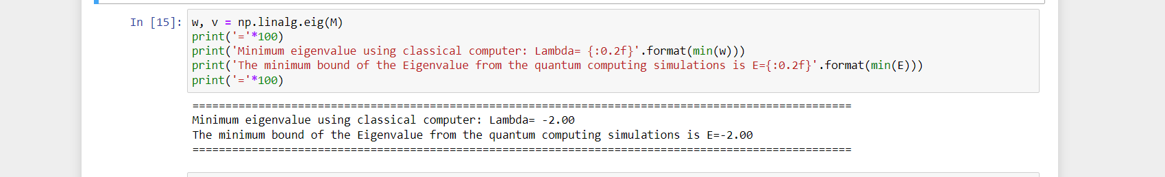
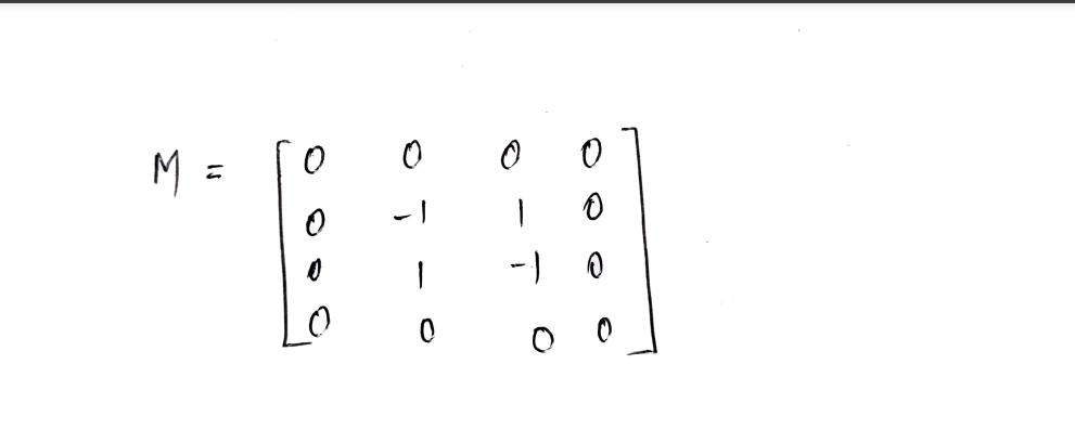
Example : Determine the lowest eigenvalue of the matrix M using the variational quantum eigensolver method (VQE).where M :

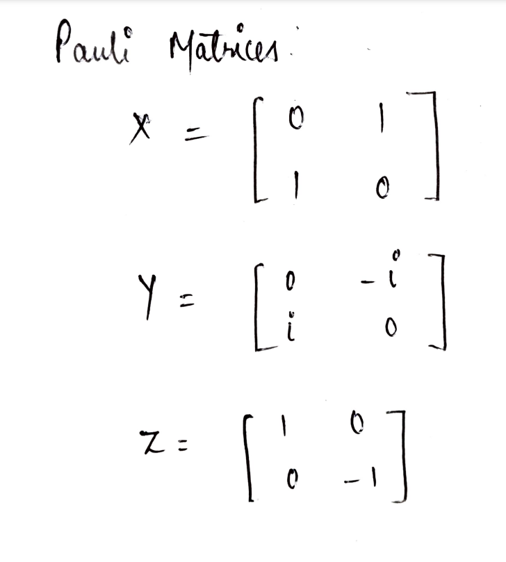
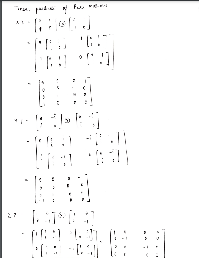
Pauli matrices are given by

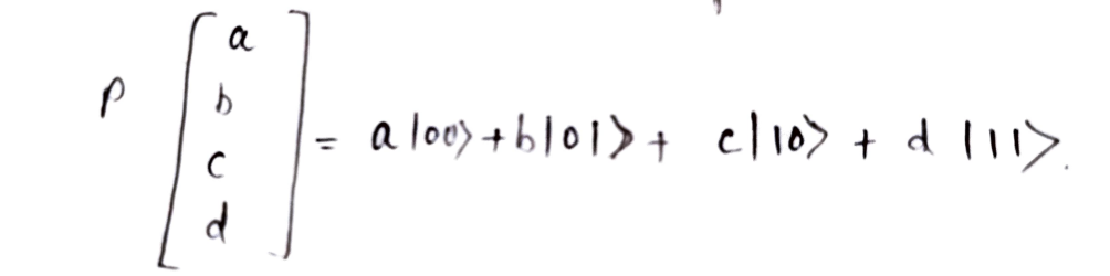
A two-qubit vector can be represented as

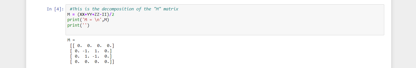
Matrix M can be  decomposed into a sum of two-qubit operators.

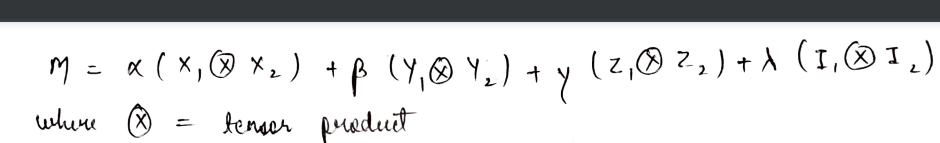
where α, β, γ, λ are unknown coeffients,

I is the identity Pauli matrix and the subscripts 1, 2 denote the qubit acted by operators.

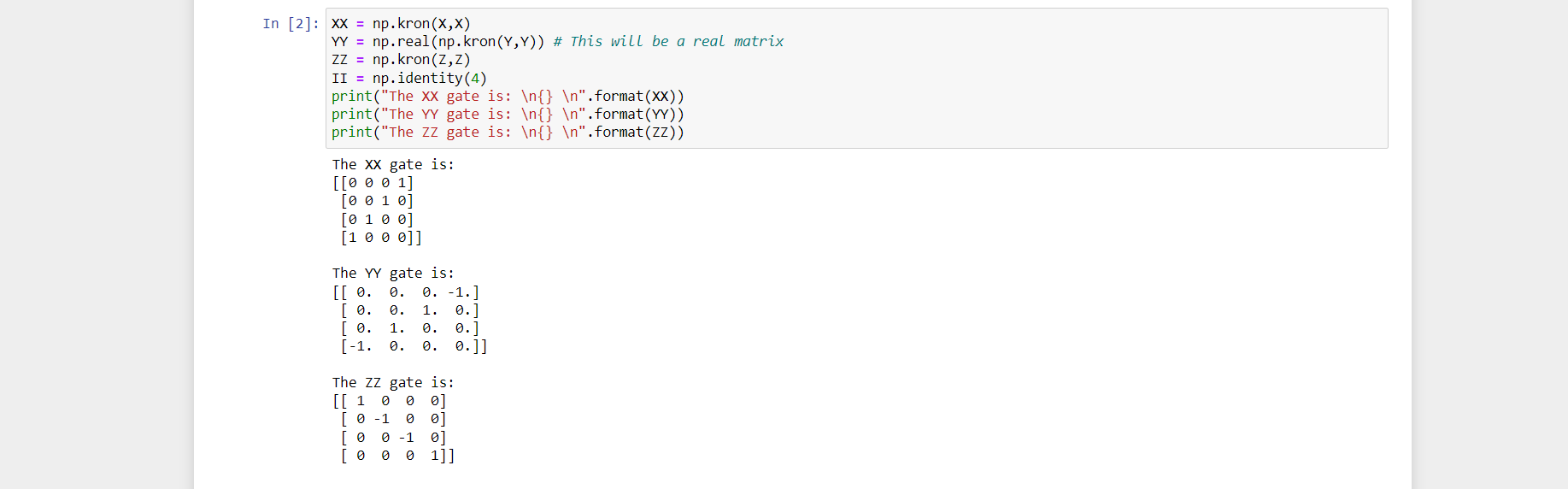
In the next step, we will create the tensor products of these operators.

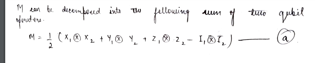
M can be decomposed into the following sum of two qubit operators.

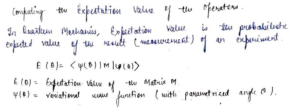
Now it is the time to determine the bound on the lowest eigenvalue of M using the variational theorem.So in order  to achieve  the solution this problem, we need to know the expectation values of M.

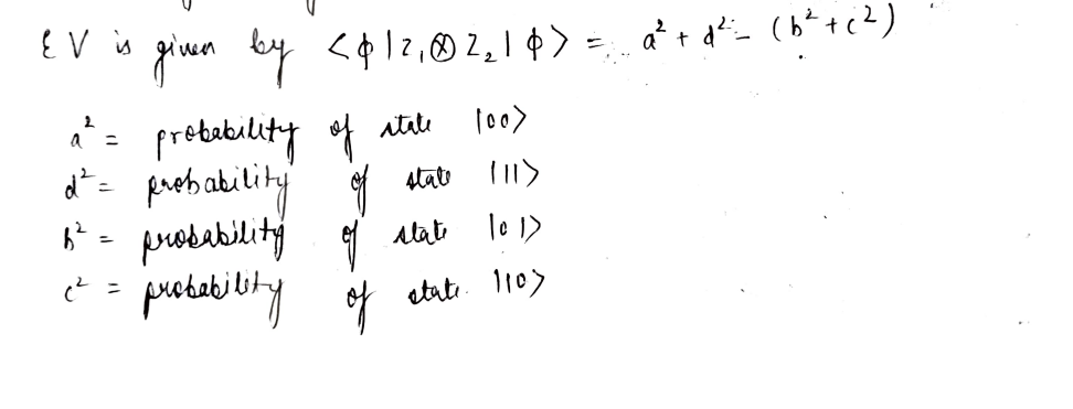
The simplest computable expectation value is the Z1 ⊗ Z2 operator. When acting on a state given by ∣ϕ⟩ = (a, b, c, d), such that ⟨ϕ|ϕ⟩ = 1, the expectation value is given by

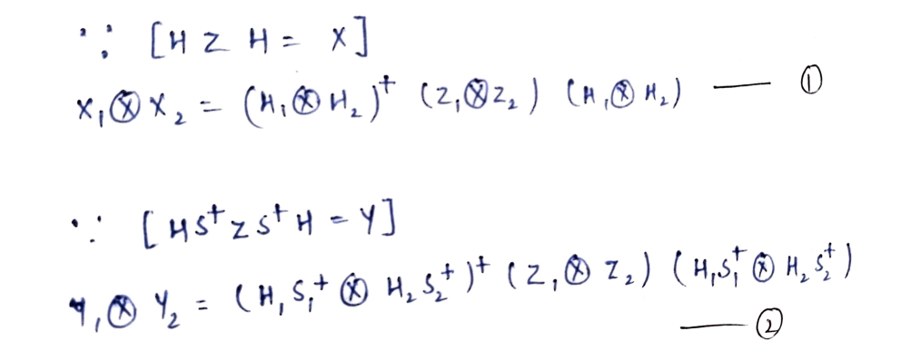
Let' determine the expectation value of other operators for the trial states,we will look into how  to decompose all two-qubit operators into the following form.

Let's do the following decompositions which is relevant to our problem.

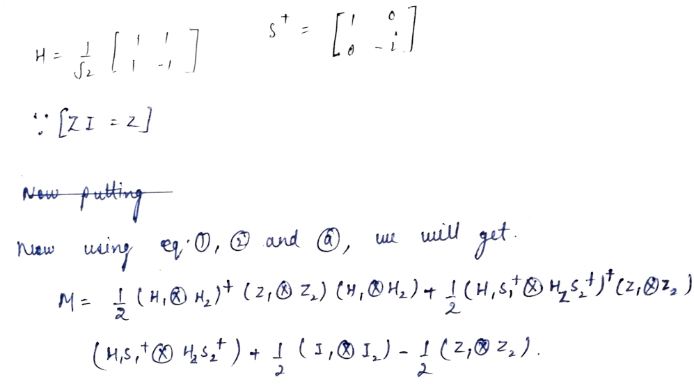
Note: The - 1/2 comes from the fact that <Ψ|II|Ψ> = 1, always a constant.

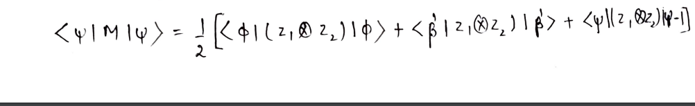
From these identities, the expectation value of the matrix M is given as

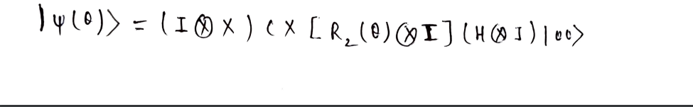
Ansatz for the VQE -

After the computation of the expectation value of the matrix M, the next step is to define a trial wave function as an ansatz.

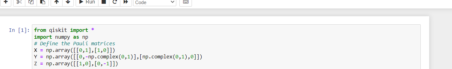
Lab implementation:

Step1:

Step2:

Step3:

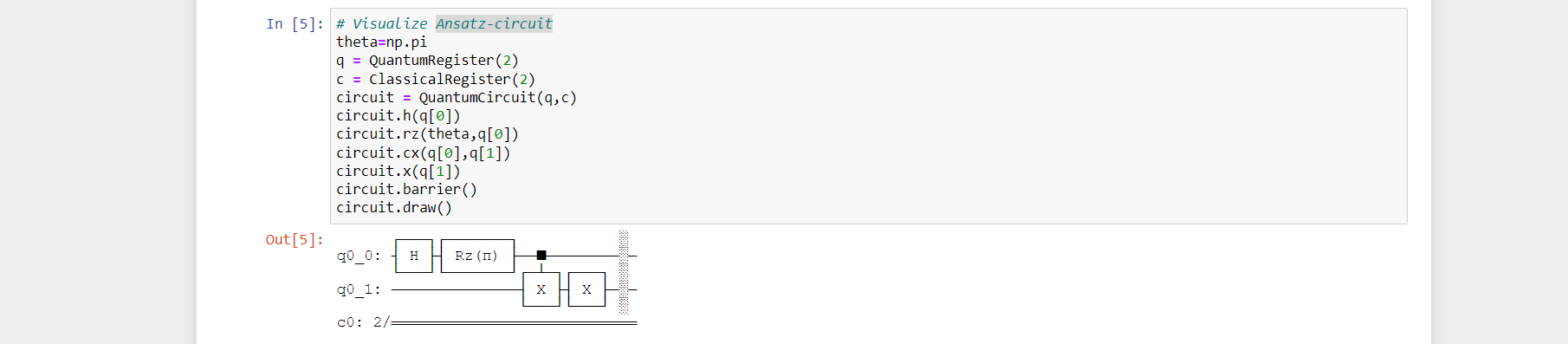
Step4: Ansatz-circuit

Step5:Let's define some functions for the evaluation of the expectation value of M

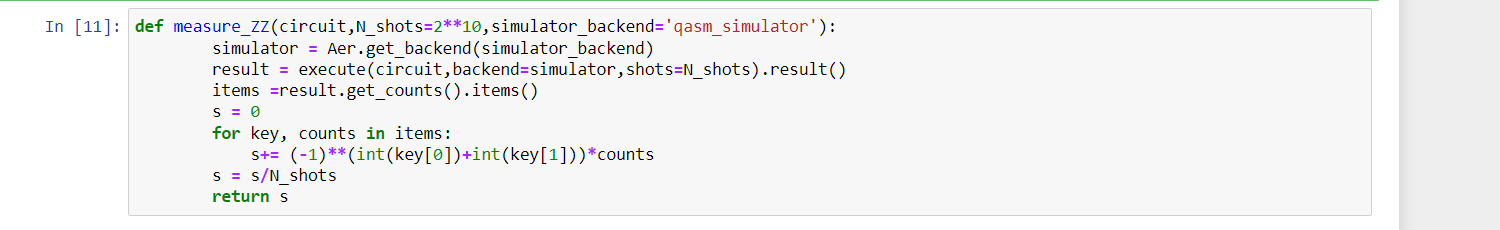
Step 6: Measures the expectation value of ZZ :

i.e. the number of ( 00 ) and (11) states, minus the number of (01) and (10) states

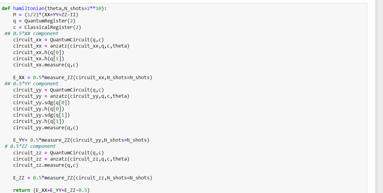
Step7: The hamiltonian is computed by separating it into three components according to the above discussion-

Step8: Generate several thetas, and find the best set of parameters and then the calculation of the expectation value of the Hamiltonian for different theta

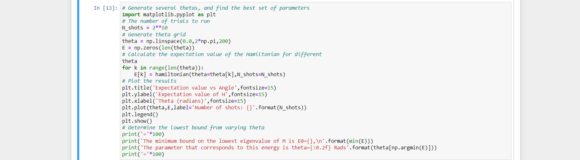
Step9:Ultimately  the plot as output determining  the lowest bound from varying theta

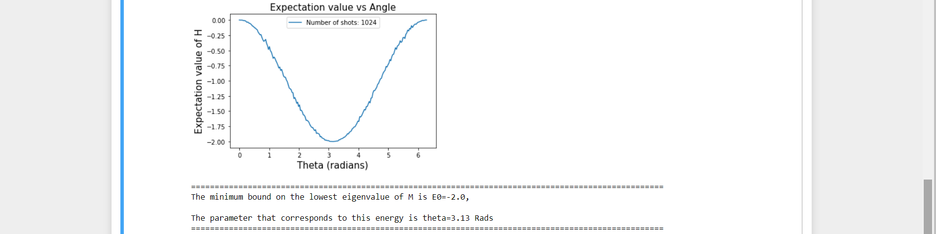
Step10:Here the output verifying that the lower bound from the quantum circuit coincides with the lowest eigen value of the matrix.