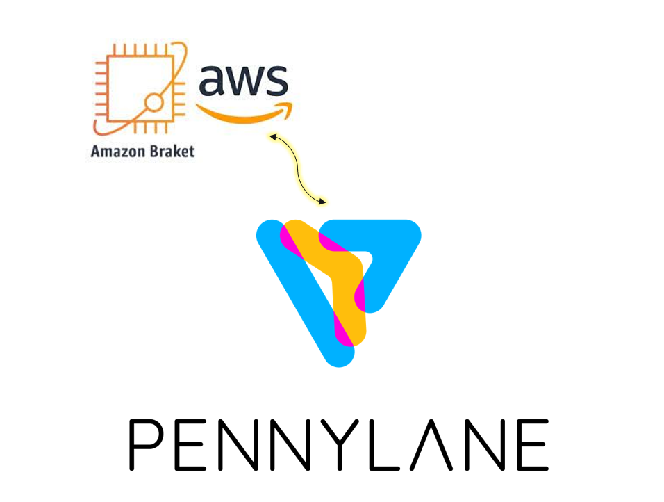
Amazon Braket Hybrid Jobs| Pennylane

HYBRID QUANTUM ALGORITHMS

Hybrid quantum algorithms are one of the most important algorithms to the industry today. Major reason is that quantum computing devices generally produce noise, and therefore, errors. Every quantum gate added to a computation increases the chance of adding noise.So long-running algorithms can be disturbed by noise, which results in inadequate computation.

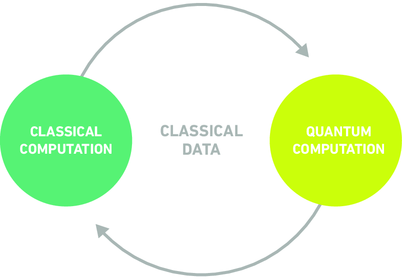
And in hybrid quantum algorithms, quantum processing units (QPUs) work as co-processors for classic CPUs, particularly to speed up certain calculations in a classical algorithm. Circuit executions become much shorter, which is in reach of the capabilities of today’s devices.

Quantum computers assured to outperform even the most-powerful classical computers on a range of computational problems for example - optimization,cryptography,material science and  chemistry . The usual set of quantum algorithms such as Shor's or Grover's quantum algorithms, specifically, these algorithms are typically believed to be feasible only with fault-tolerance as provided by quantum error correction.

In the current noisy intermediate-scale (NISQ) era, near-term quantum computers do not have a large enough number of physical qubits for the implementation of error correction protocols, and hence making this usual set of quantum algorithms unsuitable for near-term devices.So the near-term focus has been widely shifted to the class of hybrid quantum algorithms that do not require quantum error correction. In these hybrid quantum algorithms, the noisy near-term quantum computers are used as co-processors only.

QAOA(Quantum Approximate Optimization Algorithm)

There is a conventional method of finding the minimum of a binary quadratic model on a gate-based quantum computer is based on a method. And this method is called the Quantum Approximate Optimization Algorithm (QAOA). The QAOA algorithm belongs to the class of hybrid quantum algorithms (use both classical as well as quantum compute), that are widely believed to be the working for the current NISQ (noisy intermediate-scale quantum) era. In this NISQ era QAOA is also one of the best approach for benchmarking quantum devices.This can lead to practical quantum speed-up on near-term NISQ device

QUADRATIC BINARY OPTIMIZATION PROBLEMS

1) Combinatorial optimization: Combinatorial optimization problems are  across many areas of science and application areas.

for example can be found in logistics, scheduling, planning, and portfolio optimization.

2) QUBO problems: The QUBO (Quadratic Unconstrained Optimization Problem) model link to a rich variety of NP-hard combinatorial optimization problems.

for example it includes Quadratic Assignment Problems, Capital Budgeting Problems, Task Allocation Problems and Maximum-Cut Problems.

3) Maximum Cut: Among the class of QUBO problems, Maximum Cut (MaxCut) is an example of combinatorial optimization problem.

Suppose we are given a graph g=(v,e) with vertex set v and edge set e, and we basically look for partition of 'v 'into two subsets with maximum cut.

Applications can be found in, for example,

(i) clustering for marketing purposes or

(ii) portfolio optimization in finance.

Ising Hamiltonian: There is a fundamental similarity between QUBO problems and Ising problems in physics. Specifically, we can encode the Maximum Cut problem as a minimization problem of an Ising Hamiltonian, where the (classical) cost function reads

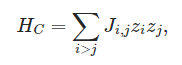
with Ising variables zi=−1,1 and the Ising matrix J encoding the weights of the edges.

In short, the cost Hamiltonian Hc assigns a number to every bitstring z=(z1,z2,…), and we would like to find the lowest number possible. This will be the optimal assignment and solution to our problem.

Amazon Braket(AWS Service)

AWS services includes one of the best services i.e.Amazon Braket. Braket is a “fully managed quantum computing service designed to help speed up scientific research and software development for quantum computing.”

Evidentaly it  provides all the quantum tools and hardware infrastructure required for new and more experienced quantum explorers to use on a pay-as-you-go basis.

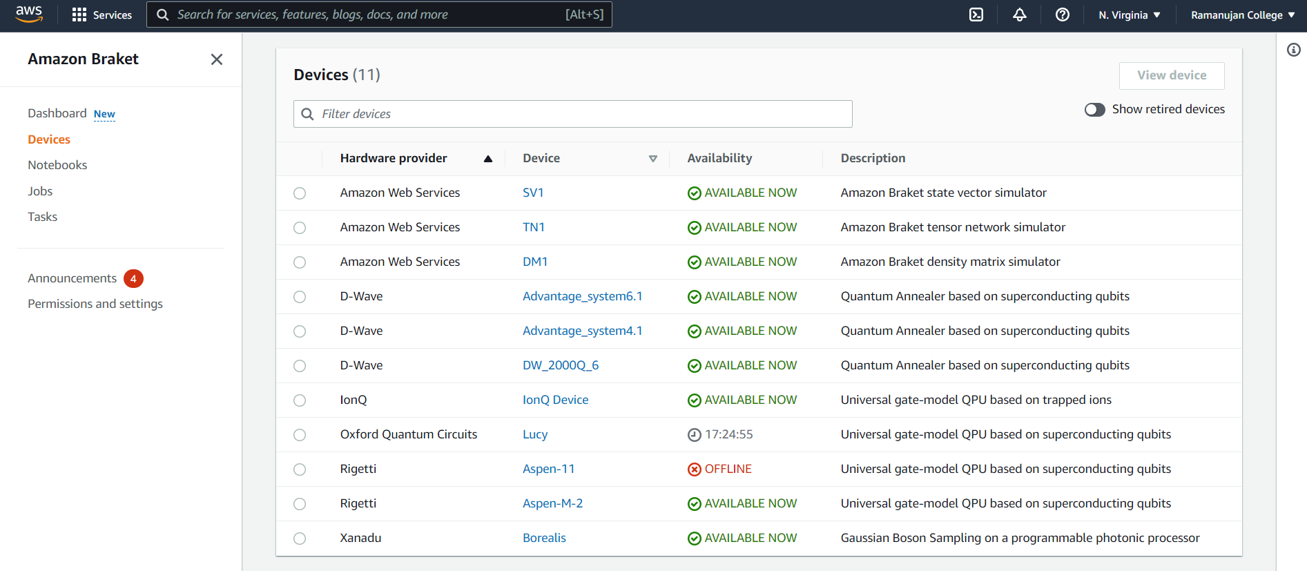
Amazon Braket currently offers access to quantum computers based on superconducting, trapped ion, photonic, and quantum annealers. You can see the list of all the available devices along with desciption and their availability and provider as shown below.

AWS has launched the Amazon Braket Hybrid late in 2021.

"Amazon Braket Hybrid Jobs enables you to easily run hybrid quantum-classical algorithms such as the Variational Quantum Eigensolver (VQE) and the Quantum Approximate Optimization Algorithm (QAOA), that combine classical compute resources with quantum computing devices to optimize the performance of today’s quantum systems. And interesting part is that with this feature, we only have to provide our algorithm script and choose a target device — a quantum processing unit (QPU) or quantum circuit simulator. Amazon Braket Hybrid Jobs is designed to spin up the requested classical resources when your target quantum device is available, run your algorithm, and release the instances after completion so you only pay for what you use. Most importantly, your jobs have priority access to the selected QPU for the duration of your experiment, putting you in control, and helping to provide faster and more predictable execution."

And in order to run a job with Braket Hybrid Jobs,  first we need to define our algorithm using either the Amazon Braket SDK or PennyLane.

Pennylane

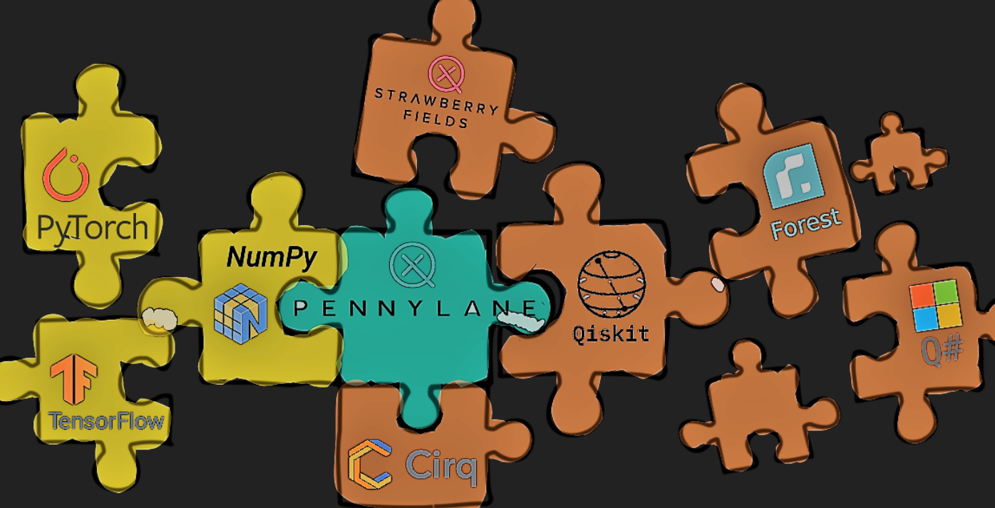
Pennylane is a cross-platform Python library for Quantum Machine Learning(QML),optimization of hybrid quantum-classical computations and automatic differentiation.

Its principal job is to manage the execution of quantum computations, including the evaluation of circuits and the computation of their gradients. This information is forwarded to the classical framework, and hence creating an ideal quantum-classical pipelines for applications.

PennyLane basically works by fusing the machine learning libraries with quantum simulators and hardware, giving users the power to train quantum circuits. And the interesting and important part is Pennylane is written in Python, so if you know Qiskit, it is not that hard to learn about PennyLane. Classical computations,optimization or training of models, are executed using the standard scientific computing or machine learning libraries such as SciPy in Python. PennyLane provides an interface to these libraries and merge these with quantum simulators to provide an interface between classical and quantum computing.

PennyLane’s uses NumPy to perform computations, but connects with machine learning libraries like PyTorch and Tensorflow for writing programs.PennyLane is built with default simulator devices, and connected with external software and hardware to run quantum circuits.

Advantage: By using PennyLane we can control and manipulate parametrized quantum circuits or variational circuits on quantum devices, and if we use PennyLane we can easy feed these circuits to quantum neural networks. Using PennyLane, we can easily find and operate gradients of quantum circuits, which is essential for the machine learning package to perform backpropagation.

As discussed above Hybrid algorithms are algorithms that contain classical and quantum instructions. The classical instructions are executed on classical hardware and the quantum instructions are executed either on a simulator or on a quantum computer.

Amazon Braket enables you to set up and run hybrid quantum algorithms with the assistance of the Amazon Braket PennyLane plugin, or with the Amazon Braket Python SDK.

Amazon Braket with PennyLane

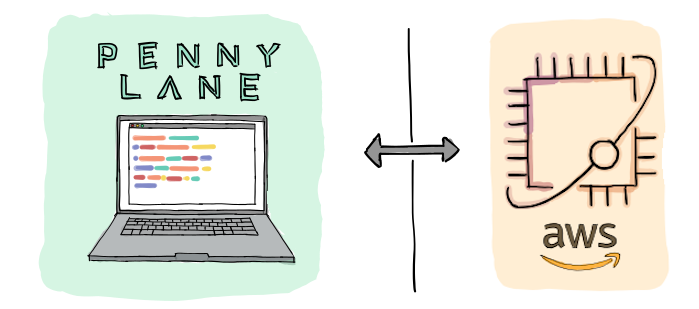
Amazon Braket allows support for PennyLane, an open-source software framework built around the concept of quantum differentiable programming. This framework provides us to train quantum circuits in the same way that you would train a neural network to find solutions for computational problems in quantum chemistry, quantum machine learning, and optimization.

The PennyLane library provides interfaces to familiar machine learning tools, including PyTorch and TensorFlow, to make training quantum circuits fast, easy and intuitive

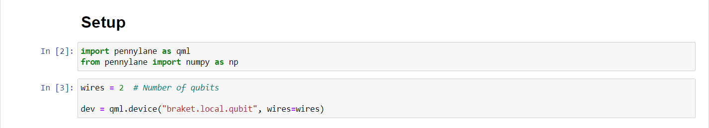
The PennyLane Library -– PennyLane is pre-installed in Amazon Braket notebooks. For access to Amazon Braket devices from PennyLane,we need to open a notebook and import the PennyLane library with this command:

 import pennylane as qml

The Amazon Braket PennyLane plugin — To use your own IDE, you can install the Amazon Braket PennyLane plugin manually. The plugin connects PennyLane with the Amazon Braket Python SDK, so you can run circuits in PennyLane on Amazon Braket devices. To install the the PennyLane plugin, use this command:

pip install amazon-braket-pennylane-plugin

The Amazon Braket PennyLane plugin enables us to switch between Amazon Braket QPU and simulator devices in PennyLane with a single line of code.

It basically offers two Amazon Braket quantum devices to work with PennyLane:

braket.aws.qubit This is use for running with the Amazon Braket service’s quantum devices, including QPUs and simulators

braket.local.qubit This is use for running with the Amazon Braket SDK’s local simulator

Quantum circuits

In PennyLane, quantum computations, which requires the execution of one or more quantum circuits, can be represented as quantum node objects. So we can say that a quantum node is used to declare the quantum circuit, and as well as it ties the computation to a specific device that executes it.

QNodes can interface with any of the supported numerical and machine learning libraries. By default, QNodes use the NumPy interface.

Using the NumPy interface

Using the NumPy interface is easy in PennyLane, and the default approach — designed so it will feel like you are just using standard NumPy, with the added benefit of automatic differentiation.

All you have to do is make sure to import the wrapped version of NumPy provided by PennyLane alongside with the PennyLane library:

        import pennylane as qml·        

        from pennylane import numpy as np

Defining a device

So in order to run and later optimize a quantum circuit, first we needs to specify a computational device.

The device is an instance of the Device class, and can represent either a simulator or hardware device. They can be instantiated using the device loader.

Device options

While loading a device, the name of the device must always be detailed out clearly. And rest additional options can then be passed as keyword arguments, and can differ based on the device.

The two most important device options are the wires and shots arguments.

Wires

This argument can either be an integer that defines the number of wires that we can address by consecutive integer labels 0,1,2,...

Shots

This argument is an integer that defines how many times the circuit should be evaluated. And also on some supported simulator devices, shots=None, computes measurement statistics exactly.

Note: This argument can be temporarily revoke when a QNode is called.

For example, my_qnode(shots=2) will temporarily evaluate my_qnode using two shots.

Creating a quantum node

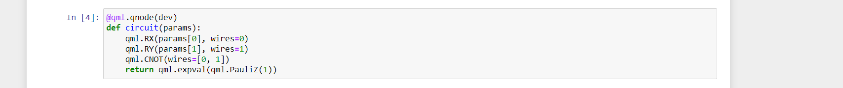
Together, a quantum function and a device are used to create a quantum node or QNode object, which wraps the quantum function and binds it to the device.

To view the quantum circuit given specific parameter values, we can use the draw() or draw_mpl() transform.

Optimizers

Optimizers are objects which can be used to automatically update the parameters of a quantum or hybrid machine learning model. We are free to use the Optimizers as per our own choice of the classical autodifferentiation library, and are available from different access points.

NumPy

And When we are using the standard NumPy framework, PennyLane offers some built-in optimizers. Some of these are specific to quantum optimization, such as the QNGOptimizer,LieAlgebraOptimizer,RotosolveOptimizer,RotoselectOptimizer, and ShotAdaptiveOptimizer.

Here are some:

1. AdagradOptimizer
   Gradient-descent optimizer with past-gradient-dependent learning rate in each dimension.

2. AdamOptimizer
   Gradient-descent optimizer with adaptive learning rate, first and second moment.

3. GradientDescentOptimizer
   Basic gradient-descent optimizer.

4. LieAlgebraOptimizer
   Lie algebra optimizer.

5. MomentumOptimizer
   Gradient-descent optimizer with momentum.

6. NesterovMomentumOptimizer
   Gradient-descent optimizer with Nesterov momentum.

   And many more

Gradients

The interface between PennyLane and automatic differentiation libraries relies on PennyLane’s ability to compute or estimate gradients of quantum circuits. There are different strategies to do so, and they may depend on the device used.

And when we create a QNode, we can specify the differentiation method like this:

@qml.qnode(dev, diff_method="parameter-shift")
def circuit(x):
       qml.RX(x, wires=0)
       return qml.probs(wires=0)

Device gradients

"device": Queries the device directly for the gradient. Only allowed on devices that provide their own gradient computation.

The return value of the QNode, e.g. qml.expval() or qml.probs()

Let's now deep dive into it by trying out some cases:-

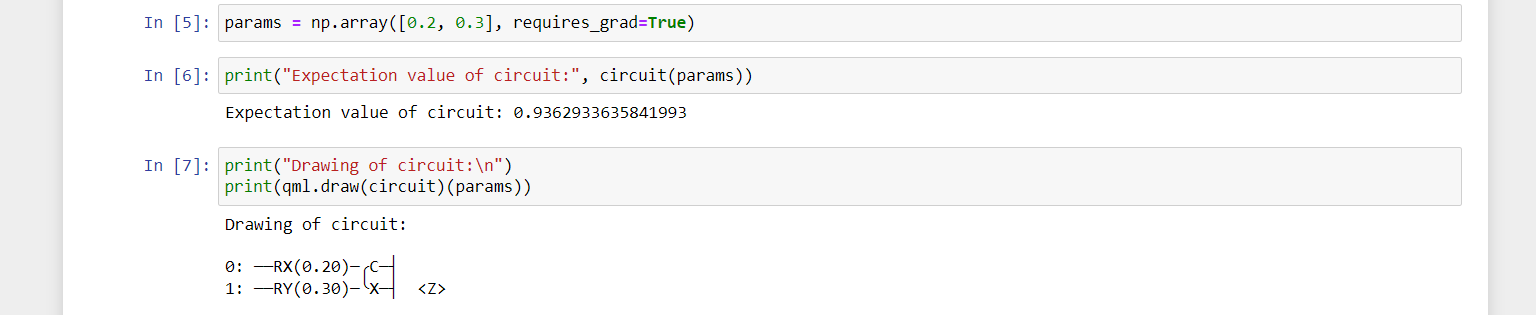
Example 1:  How to construct circuits and evaluate their gradients in PennyLane with execution performed using Amazon Braket

Step 1: Set up

Step 2: Defining a circuit

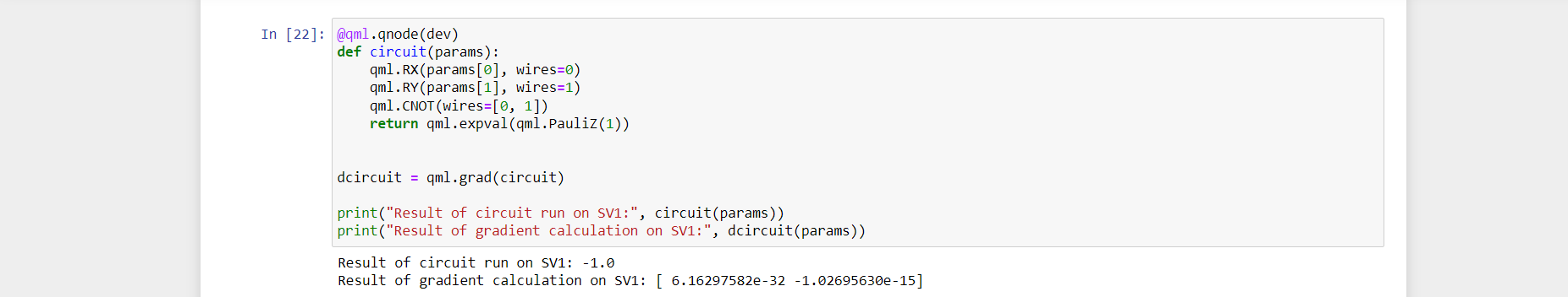
Here, chosen a simple two-qubit circuit with two controllable rotations and a CNOT gate.

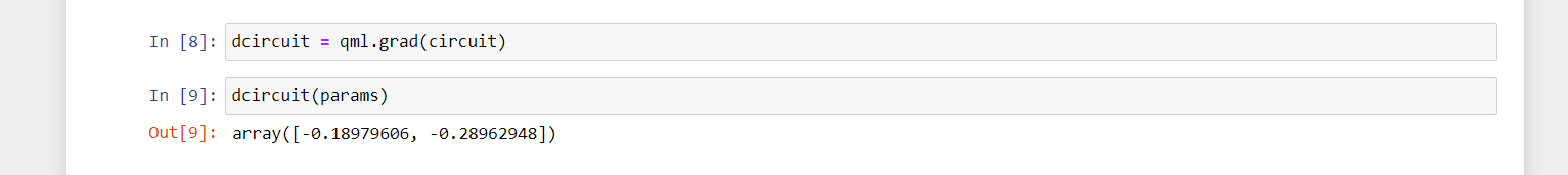
Step 3: Evaluating the circuit and accessing its gradient

A crucial element of machine learning and optimization is accessing the gradient of a model with respect to its parameters. This functionality is built into PennyLane:

Here, dcircuit is a callable function that evaluates the gradient of the circuit, i.e., its partial derivatives with respect to the controllable parameters.

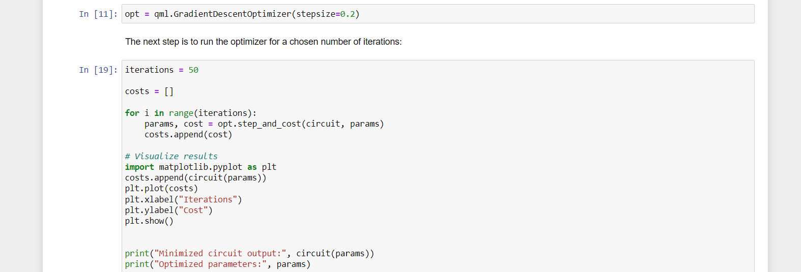
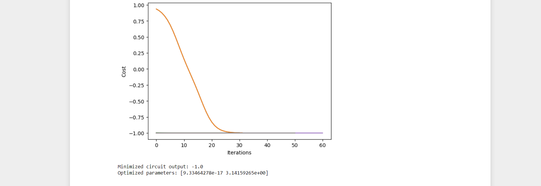
Step 4: Training the circuit

Suppose we now want to minimize the output of the circuit by updating its parameters. This can be done using gradient-based optimization.

Output:

Step 5: Running circuits on Braket's on-demand simulator, SV1

# to use SV1

s3 = ("my-bucket", "my-prefix")

sv1 = qml.device("braket.aws.qubit",

device_arn="arn:aws:braket:::device/quantum-simulator/amazon/sv1",

s3_destination_folder=s3, wires=2)

Example 2: Let's deep dive into how quantum circuit training can be applied to a problem of graph optimization. We show how easy it is to train a QAOA circuit in PennyLane to solve the maximum clique problem on a simple example graph.

Application : One application area where near-term quantum hardware is expected to shine is in graph optimization. Graph-based problems are interesting to explore because they have both strong links to practical use-cases (such as logistics and social networks) and are also often hard to solve.

Step 1 : PROBLEM SETUP

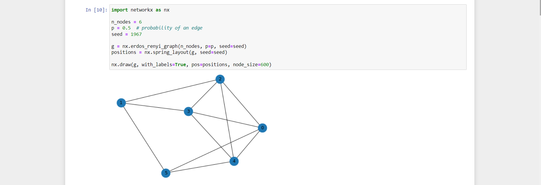
To get started, we first use the open-source networkx library to visualize the problem graph.

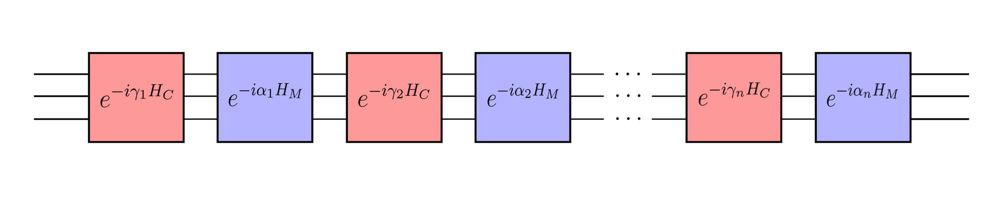
The quantum approximate optimization algorithm (QAOA) is a general technique that can be used to find approximate solutions to combinatorial optimization problems, in particular problems that can be cast as searching for an optimal bitstring. QAOA consists of the following steps

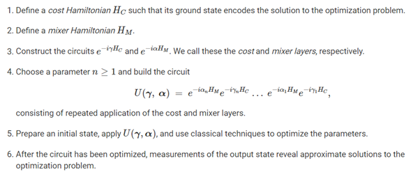
In summary, the starting point of QAOA is the specification of cost and mixer Hamiltonians. We then use time evolution and layering to create a variational circuit and optimize its parameters. The algorithm concludes by sampling from the circuit to get an approximate solution to the optimization problem.

Step 2: Fixing the problem

Let's consider the graph above and aim to find the maximum clique, i.e., the largest set of nodes that are fully connected.

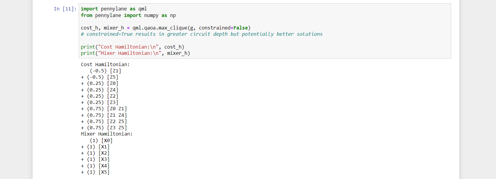
To solve this using QAOA in PennyLane and Braket, we need to first calculate the cost Hamiltonian (Hc) and corresponding mixer Hamiltonian (Hm).

Step 3 : Setting up the algorithm

-Setting up a single QAOA layer

-This layer contains the controllable parameters gamma and alpha.

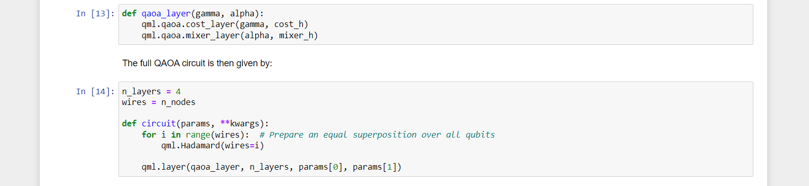
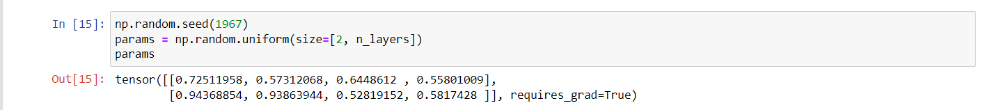
So there will be overall 8 controllable parameters: the first 4 are for of the cost Hamiltonian(Hc) and the second 4 are for of the mixer Hamiltonian(Hm):

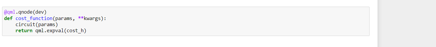
Step 4: The final step is to define the cost function. In QAOA, the output cost function is given by the expectation value of the cost Hamiltonian , i.e.,

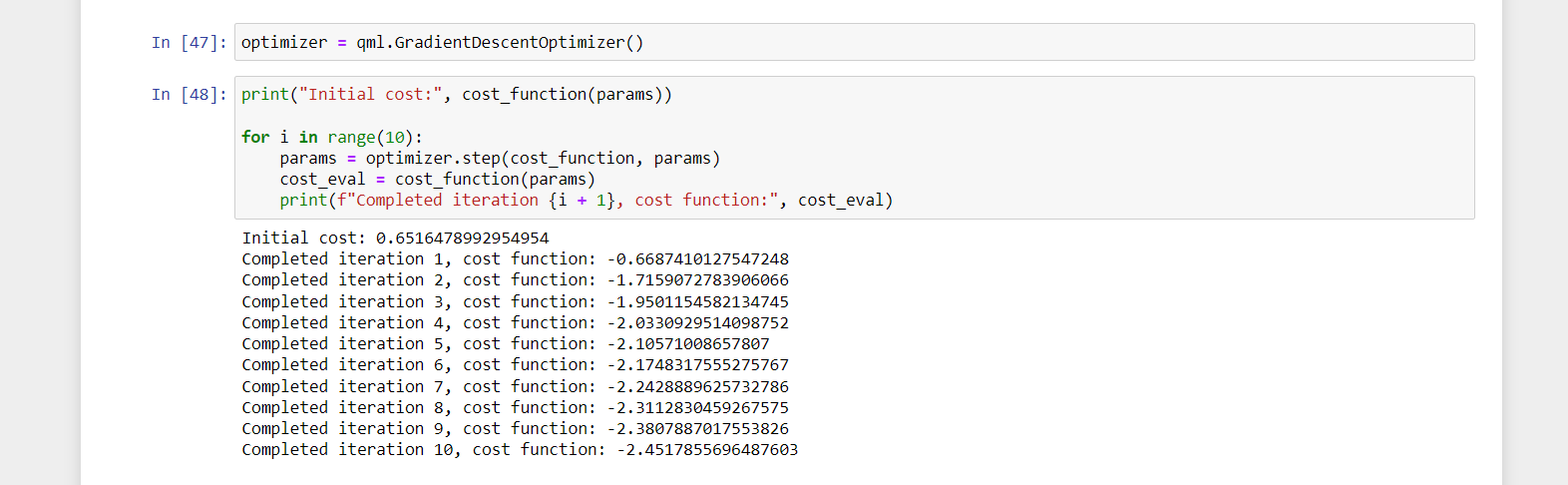
Step 5: Running the algorithm

Now that we have set up the cost function, we just need to pick an optimizer and run the standard optimization loop.

Step 6: Investigating the result

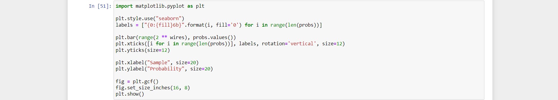
Note : We can take sample from the circuit using the optimized parameters. This will give us binary samples that allow us to select which nodes of the graph to use as part of our clique, e.g., either by simply selecting the most common sample or selecting the sample with the lowest corresponding energy.

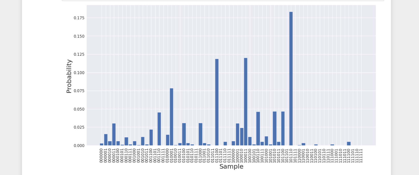
Conclusion drawn from the above graph - It is clear that the sample 101110 has the greatest probability. Since each qubit corresponds to a node, this sample selects the nodes [0, 2, 3, 4] to form a subgraph.

Okay Let's check if this is a clique, i.e., if all of the nodes are connected:

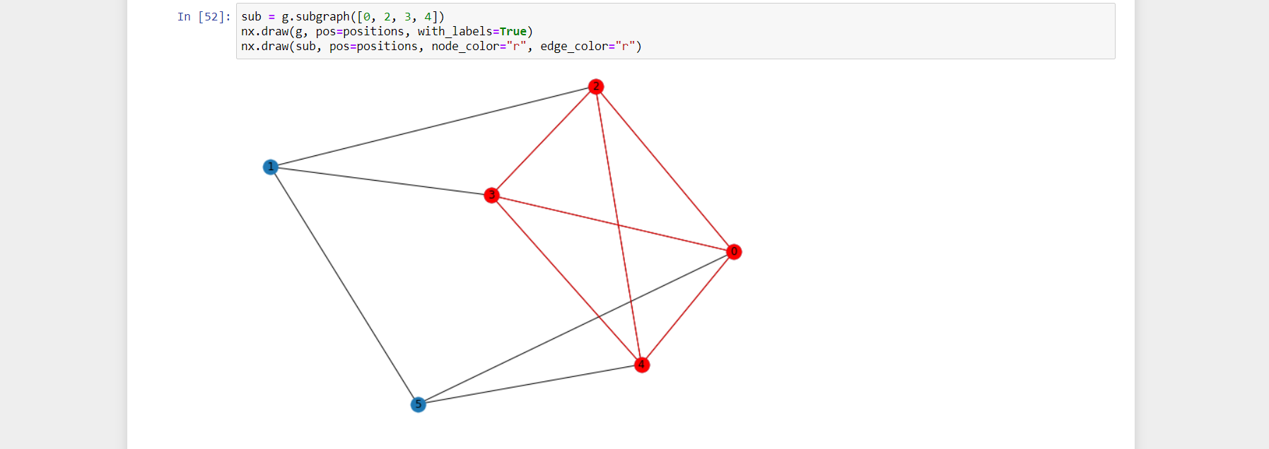
Great, this is a clique! Moreover, it is the largest clique in this six-node graph. QAOA, using PennyLane and Braket, has helped us to solve the maximum clique problem!